Zero-Downtime Summary Table Refresh Using AB Rotating Tables in Oracle Exadata and Redshift

Aside July 27, 2020 lukelushu Leave a comment

Zero-Downtime Summary Table Refresh Using AB Rotating Tables in Oracle Exadata and Redshift

1. Zero-Downtime Refresh Framework in Oracle Exadata

In Enterprise Data Warehouse system, it is quite often some summary tables are required to refresh several times even hourly per day. Meanwhile most of the summary tables are accessed globally in 24/7 mode . That is, there is no any downtime window allowed for the scheduled or on-demand refreshes. Therefore, how to implement the Zero-Downtime table refresh is a challenge.

In our Oracle Exadata-based Enterprise Data Warehouse system, we successfully developed the framework for the Summary Table Refresh process using A/B Rotating strategy to automatically implement the Zero-Downtime refresh process.

The Oracle-based framework is outlined below:

1. 1. Create A/B tables — For each of the summary tables to refresh, say a sales summary fact table named “F_SLS_SUM”, create two identical A/B tables “F_SLS_SUM_A” and “F_SLS_SUM_B” .
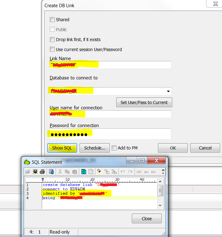
  2. Create a Public Synonym “F_SLS_SUM” pointing to one of the A/B tables appropriately and dynamically during the process.
  3. Configure and Update Refresh Control Table: REFRESH_CRTL_TAB ( Synonym_Name*, Schema_Name*, Rotate_Table_Name*, Rotate_Status, Refresh_Status).
  4. The process refresh the “Inactive” Rotate table and update the Rotate and Refresh status correspondingly (columns with * are unique). For example:

2. Zero-Downtime Refresh Implementation in Redshift

In Redshift there is no Public Synonym concept (at least at this blog writing time). Therefore we can’t migrate the existing Oracle-based Zero-Downtime refresh framework directly to Redshift by switching the Public Synonym.

As a workaround solution in Redshift, After the refresh process sync the refresh control table, rather than switch the Public Synonym, we can define a Redshift view using the Refresh Control Table :
CREATE OR REPLACE VIEW EDW.F_SLS_SUM_V AS (SELECT * FROM EDW.F_SLS_SUM_AWHERE EXISTS ( SELECT 1 FROM EDW.REFRESH_CNTRL_TAB WHERE ROTATE_TABLE_NAME ='F_SLS_SUM_A' AND ROTATE_STATUS ='ACTIVE' ) ) UNION ALL (SELECT * FROM EDW.F_SLS_SUM_B WHERE EXISTS ( SELECT 1 FROM EDW.EFRESH_CNTRL_TAB WHERE ROTATE_TABLE_NAME ='F_SLS_SUM_B' AND ROTATE_STATUS ='ACTIVE' ) );

For example,

CREATE VIEW EDWADM.F_DLY_SLS_REPT_SUM_V AS (SELECT * from EDWADM.F_DLY_SLS_REPT_SUM_A WHERE EXISTS (SELECT 1 FROM EDWADM.EDW_REFRESH_CNTRL_TAB WHERE ROTATE_TABLE_NM = 'F_DLY_SLS_REPT_SUM_A' and ROTATE_STATUS = 'ACTIVE') UNION ALL SELECT * from EDWADM.F_DLY_SLS_REPT_SUM_B WHERE EXISTS (SELECT 1 FROM EDWADM.EDW_REFRESH_CNTRL_TAB WHERE ROTATE_TABLE_NM = 'F_DLY_SLS_REPT_SUM_B' and ROTATE_STATUS = 'ACTIVE') );
In this way, the view F_SLS_SUM_V will return one of the rotating table A’s or B ‘s data, according to the rotating status of the refresh control table.

AWS, Redshift

S3 Folder Structure and Its Impacts for Redshift Table and Glue Data Catalog

Aside April 13, 2018 lukelushu Leave a comment

S3 Folder Structure and Its Impacts for Redshift Table and Glue Data Catalog

Suppose we export a very large table data into multiple csv files with the same format, or split an existing large csv files into multiple csv files. All these files are stored in a S3 bucket folder or its subfolders. We call this S3 folder the root folder of the table, or root-folder for short. In this blog we will explore the best way to organize the multiple files in the root-folder and its subfolders, so that we can easily access these files in from Redshift or discovery them in the AWS Glue catalog.

We start the experiments with four csv files (test_file1, test_file2, test_file3, and test_file4). All the files have the three fields (cust_id: integer, cust_type: text, cust_name: text), but not contains the header info. They will be organized in different S3 folder structures within the root folder “test”. Then we will observe their behaviors when we access them with Redshift and AW Glue in the three ways below:

Reload the files into a Redshift table using command “COPY”,
Create an Spectrum external table from the files
Discovery and add the files into AWS Glue data catalog using Glue crawler

We set the root folder “test” as the S3 location in all the three methods. For the Redshift, below are the commands use:

Reload the files into a Redshift table “test_csv”:

create table test_csv (cust_id integer, cust_type text, cust_nme text);

copy test_csv
from 's3://redshift-colddata/test/' 
iam_role 'arn:aws:iam::[aws-acct]/'RedshiftSpectrumRole'
delimiter ',';

Create the Redshift External Table:

create external table spectrumtest.test_csv_ext(cust_id integer, cust_type text, cust_nme text)
row format delimited fields terminated by ','
stored as textfile
location 's3://redshift-colddata/test/';

Case 1: All the 4 files are in the root folder “test”:

The S3 root folder structure:

.\test\file1
.\test\file2
.\test\file3
.\test\file4

Redshift Result:

Both the tables "test_csv" and "test_csv_ext" have all the data from the 4 files.

Glue Crawler Catalog Result:

Discoveried one table: "test" (the root-folder name). It has all the data from the 4 files, and it is not partitioned.

Case 2: Some files are in the root folder and some files in subfolders:

The S3 root folder structure:

..\test\sbf1\file1
..\test\file2
..\test\file3
..\test\file4

Redshift Result:

Both the tables "test_csv" and "test_csv_ext" have all the data from the 4 files.

Glue Crawler Catalog Result:

Discoveried four tables: (the sub-folder name and file names)
    "sbf1"  --  Only has the data from "file1". 
    "file2" --  No data found. 
    "file3" --  No data found. 
    "file4" --  No data found.

Case 3: Files are in the same level subfolders:

The S3 root folder structure:

..\test\sbf1\file1, file2
..\test\sbf2\file3, file4

Redshift Result:

Both the tables "test_csv" and "test_csv_ext" have all the data from the 4 files.

Glue Crawler Catalog Result:

Discoveried one table: "test" (the root-folder name). It has all the data from the 4 files, and it is partitioned on one coluumn into two partitions "sbf1", and "sbf2" (sub-folder names become partition values).

Case 4: Files are in the different level of the multi-level subfolders:

The S3 root folder structure:

..\test\sbf1\sbsbf11\file1
..\test\sbf1\sbsbf12\file2
..\test\sbf2\file3, file4

Redshift Result:

Both the tables "test_csv" and "test_csv_ext" have all the data from the 4 files.

Glue Crawler Catalog Result:

Discoveried two tables:
   "sbf1" -- It has the data from the two files: "file1" and "file2". it is partitioned into two partitions "sbsbf11", and "sbsbf12".
   "sbf2" --  It has the data from the two files: "file3" and "file4". It is not partitioned.

Case 5: Files are in the same level of multi-level subfolders:

S3 Folder structure:

..\test\sbf1\sbsbf11\file1
..\test\sbf1\sbsbf12\file2
..\test\sbf2\sbsbf21\file3
..\test\sbf2\sbsbf22\file4

Redshift Result:

Both the tables "test_csv" and "test_csv_ext" have all the data from the 4 files.

Glue Crawler Catalog Result:

Discoveried one table: "test" (the root-folder name). It has all the data from the 4 files, and it is partitioned on two coluumns. The partitions are 
        ["sbf1","sbf1-sbsbf11"]
        ["sbf1","sbf1-sbsbf12"]
        ["sbf2","sbf2-sbsbf21"]
        ["sbf2","sbf2-sbsbf22"]

Conclusions

From the test results above, we can conclude:

Redshift “COPY” or external table don’t care about the S3 subfolder structure and how the files are organized within the root folder or its subfolders. As long as the files have same format, the data from all the files can be accessed from the one single Redshift table or external table by specifying the S3 location as the root folder for the files, no matter where they are stored within the multi-level subfolders.
However, in order the Glue crawler to add the S3 files into the data catalog correctly, we have to follow the rules below to organize and plan the S3 folder structure.
- If you don’t want to utilize partition feature, store all the files in the root folder.
- If you want to utilize the partition feature, design the subfolder structure carefully, and always distribute the files among the subfolders at same level.
- The number of subfolder levels should be the same number of the columns to be partitioned.
- Never place the files into different level subfolders. Never mix files and folders are siblings at any level.

AWS, Redshift

Redshift Naming Standard and Case Sensitivity

Aside April 11, 2018 lukelushu Leave a comment

Redshift Naming Standard and Case Sensitivity

Everyone knows that Amazon Redshift is based on PostgreSQL. Most people think Redshift and PostgreSQL have the same or similar naming case sensitivity of the identifiers (table names and column names).

But actually Redshift and PostgreSQL have a number of very important differences in the naming standard and case case sensitivity that you must be aware of as you work with Redshift.

Basically, in Redshift there are two types of Identifiers: Standard Identifiers and Double-quoted Identifiers. The identifier types are distinguished when they are created in the DDL script with or without the double-quote marks. The AWS document Names and Identifiers defines the naming rules for these two types of identifiers (table names and column names).

In general, in Redshift the UTF-8 multibyte characters two or four bytes long are allowed in the identifier names. In practice, let’s limit the identifier names to use single-byte ASCII characters only in this blog.

Standard Identifiers Rule

There are three simple rules for the Standard Identifiers:

Begin with an alphabetic character or underscore, followed by any ASCII alphanumeric characters, underscores, or dollar signs.
Not be a reserved SQL key word, like group, user.
Be between 1 and 127 characters in length.

The first rule implies that the identifier name should not contain any spaces or quotation marks.

Double-quoted Identifiers Rule

There are also three simple rules for the Double-quoted Identifiers:

Begin and end with double-quote marks (“).
The identifier can contain any ASCII printable characters, including the spaces and even the double-quote mark (“) itself.
Be between 1 and 127 characters in length.

Notes:

You can use the reserved SQL key word like group, user, etc. as the table name or column name, but they have to be double-quoted.
You even can include the double-quote mark (“) itself in the table or column names. But it must be escaped by preceding with another double-quote mark (“).

Database Catalog and Reference of the Identifiers

After creating the objects with the standard Identifiers or double-quoted Identifiers or their mixture, how to use them?

Different databases have different ways to store the identifiers in the database catalog and reference them.

In Redshift, all ASCII letters in the identifiers (for both the standard and double-quoted identifiers) are case-insensitive and are folded to lowercase in the Redshift Catalog.

The identifiers can be referenced in the following simple and convenient ways:

For the Standard Identifiers, they can be referenced in any letter-case or mixture, with or without the double-quote marks.
For the Double-Quoted Identifiers,
- If the quoted part meet the Standard Identifiers rules, then it can be referenced in any letter-case, with or without the paired double-quote marks. Just like the Standard Identifiers.
- Otherwise, you must use the double quotation marks for every reference to that identifier, all ASCII letters can be any case, but the others should be exactly the same as it was defined.

Want to Return the Identifiers to Upper Case?

As said before, all ASCII letters in the identifiers (for both the standard and double-quoted identifiers) are are stored in the database catalog as lowercase . Therefore, in query results, all the column names are returned as lowercase by default. If you want to return all the column names in uppercase, set the describe_field_name_in_uppercase configuration parameter to true.

set describe_field_name_in_uppercase to on;
show describe_field_name_in_uppercase;

Then you will see all the return column names are in upper case. Remember, the column names in catalog are still in lowercase.

Examples

The following is a valid DDL to create a table

create table "TEst_TaBle1"(cOLuMN1 text, "coLuMn #2" text, "coLuMn ""3""" text);

Then table name and column names in the catalog will be

test_table1 (column1, column #2, column "3" )

The following queries are valid and will return the same result:

select   COLUMN1,  "COLumn #2",  "COLumn ""3""" from  TEst_TaBle1;
select "colUmn1",  "coLUmn #2",  "columN ""3""" from "teST_taBLE1";
select  column1,   "colUMN #2",  "COLumn ""3""" from "Test_taBLE1;

IAM

How to Assume IAM Role From AWS CLI

Aside March 19, 2018 lukelushu Leave a comment

How to Assume IAM Role From AWS CLI

You can fellow the following 3 steps to assume an IAM role from AWS CLI:

Step 1: Grant an IAM user’s privilege (permission) to assume an IAM role or all IAM roles
Step 2: Grant a particular IAM role to the IAM user. That is, modify a particular IAM role’s trust relationship to allow the IAM user to assume this role
Step 3: Configure and use the AWS CLI profile to assume the granted role

1. Grant an IAM user’s privilege:

Create a new or pickup an existing IAM user (say named it as “userTest”) with the security credentials (Access Key ID and Secret Access Key) . Note done its user ARN (like arn:aws:iam::123456789012:user/userTest).
Create a assuming role policy: It can be a generic policy (named it as “Assume-Roles”) to assume any IAM roles with the following custom policy code

{
"Version": "2012-10-17",
"Statement": [
{
"Sid": "",
"Effect": "Allow",
"Action": "sts:AssumeRole",
"Resource": "*"
}
]
}

Or you can specify a particular role’s ARN (like “arn:aws:iam::123456789012:role/roleTest”) for the Resource above to limit the policy only applicable to the IAM role named role “roleTest” and name the policy as “”Assume-Role-roleTest”.

Attach the policy to the user “userTest”.

2. Grant an IAM role to an IAM user:

Create a new or pickup an existing IAM role (say it is named as “roleTest”) with the required permissions. Note down its role ARN (like arn:aws:iam::123456789012:role/roleTest).
Modify the role’s trust relationship to add the the IAM user to the Trusted entities:

{
"Effect": "Allow",
"Principal": {
"AWS": "arn:aws:iam::123456789012:user/userTest"
},
"Action": "sts:AssumeRole"
}

3. Configure and use the AWS CLI profile to assume the granted role :

Edit the config file at ~/.aws/config to add a profile for each of the user userTest and the role “roleTest”:

[profile userTest]
region=us-east-1
output=json

[profile roleTest]
region=us-east-1
output=json
role_arn = arn:aws:iam::123456789012:role/roleTest
source_profile = userTest

If the user “userTest” is using the default profile, the source_profile line can be set to the default profile: “source_profile = default” .

Use the AWS CLI to assume the role: Call and AWS CLI commend using the profile option:

aws AnyEligibleCLICommend --profile roelTest

This will login into AWS using userTest’s security credential and then assume the IAM role “roleTest” to execute the CLI commend.

For example, suppose the user “userTest” uses the default profile, and itself does not have the Redshift access permission but the roleTest does.

If you run the AWS commend:

aws redshift describe-clusters

It will throws “not authorized” error. But if you run the AWS CLI commend:

aws redshift describe-clusters --profile roleTest

It will be successful.

Database Oracle

How To Create A Dynamic Hierarchy Tree from Flatten Parent-Child BOM Table

September 28, 2017 lukelushu Leave a comment

Let’s say we have the following flatten-out recursive Parent-Child table “HIER_NODE” to store the hierarchy Parent-Child nodes data:

hier_node(node_id, node_nm, parent_node_id, parent_node_nm)

Make sure the unique ROOT record (0, ‘Root’, Null, Null) exists. Assuming the maximum recursive depth is 10. Then the following Oracle SQL code can quickly build the dynamic 10-level Hierarchy Tree View from the hierarchy BOM table:

create or replace view hier_tree_v 
as
with  node_hier_tree as
    (
    select unique
           level as hier_level,
           sys_connect_by_path (node_id, '>') as hier_id_path,
           sys_connect_by_path (node_nm, '>') as hier_nm_path,
           decode (connect_by_isleaf,  0, 'N',  1, 'Y',  'X') as bottom_flg,
           node_id as bottom_node_id,
           node_nm as bottom_node_nm
      from hier_node
      start with node_id = 0
      connect by nocycle (prior node_id = parent_id
    )
select
    bottom_node_id as hier_base_id,
    bottom_node_nm as hier_base_nm,
    hier_level - 1 as hier_level,
    hier_id_path as hier_id_path,
    hier_nm_path as hier_nm_path,
    regexp_substr (hier_id_path, '[^>]+', 1, 1 ) as hier_id_lvl_01 , regexp_substr (hier_nm_path, '[^>]+', 1, 1 ) as hier_nm_lvl_01 ,
    regexp_substr (hier_id_path, '[^>]+', 1, 2 ) as hier_id_lvl_02 , regexp_substr (hier_nm_path, '[^>]+', 1, 2 ) as hier_nm_lvl_02 ,
    regexp_substr (hier_id_path, '[^>]+', 1, 3 ) as hier_id_lvl_03 , regexp_substr (hier_nm_path, '[^>]+', 1, 3 ) as hier_nm_lvl_03 ,
    regexp_substr (hier_id_path, '[^>]+', 1, 4 ) as hier_id_lvl_04 , regexp_substr (hier_nm_path, '[^>]+', 1, 4 ) as hier_nm_lvl_04 ,
    regexp_substr (hier_id_path, '[^>]+', 1, 5 ) as hier_id_lvl_05 , regexp_substr (hier_nm_path, '[^>]+', 1, 5 ) as hier_nm_lvl_05 ,
    regexp_substr (hier_id_path, '[^>]+', 1, 6 ) as hier_id_lvl_06 , regexp_substr (hier_nm_path, '[^>]+', 1, 6 ) as hier_nm_lvl_06 ,
    regexp_substr (hier_id_path, '[^>]+', 1, 7 ) as hier_id_lvl_07 , regexp_substr (hier_nm_path, '[^>]+', 1, 7 ) as hier_nm_lvl_07 ,
    regexp_substr (hier_id_path, '[^>]+', 1, 8 ) as hier_id_lvl_08 , regexp_substr (hier_nm_path, '[^>]+', 1, 8 ) as hier_nm_lvl_08 ,
    regexp_substr (hier_id_path, '[^>]+', 1, 9 ) as hier_id_lvl_09 , regexp_substr (hier_nm_path, '[^>]+', 1, 9 ) as hier_nm_lvl_09 ,
    regexp_substr (hier_id_path, '[^>]+', 1, 10 ) as hier_id_lvl_10 , regexp_substr (hier_nm_path, '[^>]+', 1, 10 ) as hier_nm_lvl_10
from node_hier_tree;

If you need more levels, simply extend the code.

Database Oracle

Use Oracle Warp Utility to Hide the Source Code of Packages, Procedures, Functions and Views

May 17, 2016 lukelushu Leave a comment

PL/SQL Wrap Utility for Encryption

The wrap utility (wrap.exe) provides a way for PL/SQL developers to protect their intellectual property by making their PL/SQL code unreadable. It helps to protect the source code from business competitors and others who might misuse it. For Oracle 10g or later versions, wrap.exe is shipped with Oracle client instillation and available at the directory of $ ORALCE_HOME\bin.

Wrapped source files can be moved, backed up, and processed (executed) by SQL*Plus and the Import and Export utilities, but they are not visible through the static data dictionary views *_SOURCE.

Steps of Wrapping Packages/Procedures/Functions

Develop the Packages/Procedures/Functions as usual. Test and save the source code in a file (for package, save the spec and body in separate files).
Run the warp utility to wrap the source code:

$ORACLE_HOME\bin\warp iname=sourceFile   [oname=warppedFile]

Distribute/delivery the wrapped file.

The wrapped file is is a text file, which you can run just as any script in SQL*Plus to set up your PL/SQL subprograms and packages. For example, run a wrapped file as follows:

SQL> @warppedFile

The following CREATE OR REPALCE statements are wrapped:

CREATE [OR REPLACE] FUNCTION function_name
CREATE [OR REPLACE] PROCEDURE procedure_name
CREATE [OR REPLACE] PACKAGE package_name
CREATE [OR REPLACE] PACKAGE BODY package_name
CREATE [OR REPLACE] TYPE type_name AS OBJECT

However, the CREATE[ORREPLACE]TRIGGER statement, and [DECLARE] BEGIN-END anonymous blocks, are not wrapped.

Guidelines for Wrapping

Wrap only the body of a package or object type, not the specification.
Wrap code only after you have finished editing it. Either wrap your code after it is ready to ship to users or include the wrapping operation as part of your build environment.
To change wrapped PL/SQL code, edit the original source file and then wrap it again.
Before distributing a wrapped file, view it in a text editor to be sure that all important parts are wrapped.
Notes: Wrapped PL/SQL units are upward-compatible between Oracle Database releases, but are not downward-compatible. For example, you can load files processed by the V11.1.5 wrap utility into a V11.1.6 Oracle Database, but you may not load files processed by the V11.1.6 wrap utility into a V11.1.5 Oracle Database.

Wrapping Oracle Views

As we see above, if we want to hide the source or logic of Oracle (for example, to prevent others to change the view logic. we can’t use the wrap utility on the view directly. As work-round solution, we can create an Oracle pipelined function to implement the view logic. Then use the wrap utility to encrypt the pipelined function. Finally create the view by selecting ALL from the pipelined function.

In case we need to encrypt multiple views, we can create a package containing multiple pipelined functions to implement the corresponding views’ logic. Then we just need to warp one package. Below is the pseudo-code:

For the Package spec file:

create or replace  package  views_wrap_pkg
   type  t_view1_cols  is record 
      (col1   varchar2(30 char),
       col2   integer );
   type t_view1_tab  is table of  t_view1_cols;
   function view1 return t_view1_tab  pipelined;
end views_wrap_pkg;

For the Package body file:

create or replace package body views_wrap_pkg

function view1 return t_view1_tab  pipelined as
cursor view1_cursor is
select  field1 as col1, field2 as col2 from tables ....
begin
for view1_row  in view1_cursor loop
pipe row (view1_row );
end loop;
return;
end  view1;
end views_wrap_pkg;

Warp the package body file (not warp the package spec file) and execute it.

Finally, Create the views from the encrypted package:

create or replace view test_view as select * from table(views_wrap_pkg.view1);

In this way, all the view logic is encrypted.

Database Oracle

A Oracle Function To Parse Delimited Text String Into Collection of String Tokens

May 11, 2016 lukelushu Leave a comment

We define a simple Oracle function to parse the delimited text string into a collection of sting tokens, which can be used for further processing:

First, we need define a new type of nested-table:

CREATE OR REPLACE TYPE T_STRING_TAB IS TABLE OF VARCHAR2(1000);

Next, we create the pipeline table function called “PARSE_DELMITED_TEXT”. It takes two parameters:

P_TEXT: the delimited text string to parse
P_DELIMITOR: the delimitor used in the text string

CREATE OR REPLACE FUNCTION PARSE_DELMITED_TEXT (P_TEXT VARCHAR2, P_DELIMITOR VARCHAR2) RETURN T_STRING_TAB PIPELINED
AS

CURSOR TOKEN_CURSOR IS
SELECT TRIM( REGEXP_SUBSTR (TEXT, ‘[^’||P_DELIMITOR||’]+’, 1, LEVEL) ) AS VAL
FROM (SELECT P_TEXT AS TEXT FROM DUAL )
CONNECT BY LEVEL <= REGEXP_COUNT(TEXT,'[‘||P_DELIMITOR||’]+’)+1;

BEGIN
FOR TOKEN IN TOKEN_CURSOR LOOP
PIPE ROW (TOKEN.VAL);
END LOOP;
RETURN ;
END;

That is it! You can test it very easily from SQL :

SELECT * FROM TABLE(PARSE_DELMITED_TEXT ( ‘A,B, X, Y, ABC, ‘, ‘,’));

Database Oracle

Oracle Automatic Refresh Materialized View

October 10, 2014 lukelushu Leave a comment

In Oracle Database, we can very easily create materialized views (MVs) and let Oracle handle the refresh automatically.

For example, using the following statement we can create a MV in the schema EDWCM and tell Oracle not build it now until 5:00 PM today, and then complete refresh it at 1:00 PM every Sunday.:


CREATE MATERIALIZED VIEW EDWCM.MV_CLV_RESULT_WKLY
TABLESPACE EDWCM_DATA PARALLEL 8 
-- BUILD IMMEDIATE
BUILD DEFERRED
REFRESH COMPLETE 
START WITH ( TRUNC (SYSDATE) + 17/24 ) 
NEXT ( NEXT_DAY(TRUNC(SYSDATE), 'SUNDAY') + 13/24 )
AS
[Your-MV-Select-Query go here];

After creating the automatic refresh MV, you can change the refresh time and frequency by altering the MV. For example, if you refresh it at 1:00 AM everyday, you can issue the following MV alter statement:

ALTER MATERIALIZED VIEW EDWCM.MV_CLV_RESULT_WKLY
 REFRESH COMPLETE
 NEXT (TRUNC (SYSDATE+1) + 1/24 );

Oracle is still using the deprecated Oracle Job (at least up the version 11gR2) to maintain the refresh, not use the advanced Oracle SCHEDULER. So when you create a Oracle automatic refresh MV using the syntax above, Oracle will create a Oracle job for you and schedule the job to run. You can use the following query to find the Oracle job information (write down the job_id and you will need job_id to stop or resume the automatic refresh, see below):

select * from  dba_jobs where SCHEMA_USER = 'EDWCM';

You also can use the following query to find all the refresh history in past:

SELECT * FROM dba_snapshot_refresh_times where owner = 'EDWCM';

Finally, you can stop the automatic refresh or resume the automatic refresh for the MV by (your need to supply the job_id integer value for the MV refresh job :

-- Stop the automatic refresh 
exec DBMS_JOB.BROKEN (job_id,  TRUE );

-- Resume the automatic refresh 
exec DBMS_JOB.BROKEN (job_id,  FALSE );

Notes: In order to create the automatic refresh MV, the owner of the MV should be granted the SELECT privilege directly on all the master tables (tables used in the query). The indirect grant (e.g. the grant through roles) will not not work.

Machine Learning

Support Vector Machines (2)

September 10, 2014 lukelushu Leave a comment

Linear Separability: What is the best $\Theta$ ?

In the blog Support Vector Machines (1), the SVM is formulated the as a Quadratic Programming optimization problem:

$\displaystyle \min_{\theta_0,\theta_1,...,\theta_n} \frac{1}{2}\sum_{j=1}^n\theta_j^2 = \frac{1}{2}||\theta||^2$

s.t. $(2y_i -1)\theta^TX_i \ge 1, i=1,2,...,m.$

However, consider the two scenarios below:

A. The points can be linearly separated correctly but there is a very narrow margin.
B. But possibly the large margin solution is better, even though one constraint is violated

Even more worse, the points are linearly non-separable (see figure below). What should we do?

In general there is a trade off between the margin and the number of mistakes on the training dataset. Let’s examine some possible ideas of the trade off.

Learning Maximum Margin with Noise

Possible Ideas:

Idea 1:

Find minimum $||\Theta^2||$ , while minimizing the number of training set errors. That is,

Minimize $||\Theta||^2$ + C (#train errors), where C is the Tradeoff parameter.

It sounds intuitive. However, it can’t be expressed as a Quadratic Programming problem. Solving it may be too costly.

Idea 2:

Find minimum $||\theta||^2$ , while minimizing the distance of error points to their correct hyper-plane. That is,

Minimize $||\theta||^2$ + C (total distance of error points to their correct hyper-plane)

In order to figure out the distance of error points, we introduce the “slack” variables or “noise” variables $\xi_i \ge 0, i=1,2,...,m$ for each training data points and modify the constraints as:

s.t. $(2y_i -1)\theta^TX_i \ge 1-\xi_i, i=1,2,...,m.$

We observe that

If the data point is a support vector, i.e. it is on the hyper-plane, then $\xi =0$ .
If the data point is in the margin zone but in the right side (margin violation but right), then $0<\xi \le 1$ .
If the data point is in the margin zone but in the wrong side (margin violation and wrong), then $1 < \xi < 2$ .
if the data point is totally misclassified, then $\xi > 2$ .

Then we can rewrite the problem as:

$\displaystyle \min_{\theta_0,\theta_1,...,\theta_n; \xi_1,\xi_2,...,\xi_m}||\theta||^2 + C \sum_{i=1}^m \xi_i$

s.t. $(2y_i -1)\theta^TX_i \ge 1-\xi_i, i=1,2,...,m.$

Where $C$ is is a regularization parameter with the following properties:

Small C allows constraints to be easily ignored ==> Large margin
Large C makes constraints hard to ignore: ==> Small margin
$C=\infty$ enforces all constraints: ==> Hard margin

This is still a quadratic optimization problem and there is a unique minimum.

SVM cost functions from logistic regression cost functions

We can modifiy the logistic regression learning algorithm little bit to get SVM. Recall that for the regularized logistic regression, we have the penalized cost function

$\displaystyle J(\theta) = \frac{1}{m}\sum_{i=1}^m [-y_i\log (h(\theta, X_i))-(1-y_i)\log (1-h(\theta,X_i))] +\lambda\sum_{j=1}^{n}\theta_j^2$

Where

$\displaystyle h(\theta, X) = S(\theta^TX) = \frac{1}{1+e^{-\theta^TX}}$

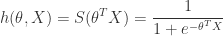
and $S(t)$ is the the Sigmoid function:

Replacing the sigmoid function into the cost function above, we have

$\displaystyle J(\theta)=\frac{1}{m}\sum_{i=1}^m [-y_i\log \frac{1}{1+e^{-\theta^TX_i}} -(1-y_i)\log \left ( 1-\frac{1}{1+e^{-\theta^TX_i}} \right )] +\lambda\sum_{j=1}^{n}\theta_j^2$

Usually we refer to the first part of the objective function as the “Training Error” which is determined by the cost function

$\displaystyle \text{Cost}(\theta, X, y) = -y\log \frac{1}{1+e^{-\theta^TX}} -(1-y)\log \left ( 1-\frac{1}{1+e^{-\theta^TX}} \right )$

and the second part as the “Complexity Term” or “Regularization term”.

From the following function plots below, we can linearly approximate the functions

$\displaystyle -\log \frac{1}{1+e^{-z}} \approx \begin{cases}1-z, & \text{ if } z < 1 \\ 0 , & \text{ if } z \ge 1\end{cases} = \max\{0, 1-z\}$

$\displaystyle -\log \left ( 1-\frac{1}{1+e^{-z}} \right ) \approx \begin{cases}0, & \text{ if } z < -1 \\1+z,& \text{ if } z \ge -1\end{cases} = \max\{0, 1+z\}$

Therefore, the cost function can be approximated as

$\displaystyle \text{Cost}(\theta, X, y) = y \max\{0, 1-\theta^TX\} + (1-y) \max\{0, 1+\theta^TX\}$

That is

$\displaystyle \text{Cost}(\theta, X, y) = \max\{0, 1- (2y-1)\theta^TX\}$

Recall the constraint $(2y_i-1)\theta^TX_i\ge 1-\xi_i$ , together with $\xi_i\ge 0$ , is equivalent to

$\xi =\max\{0, 1- (2y-1)\theta^TX\}$

Hence the SVM learning problem is equivalent to the unconstrained optimization problem over $\theta$ :

$\displaystyle \min_{\theta_0,\theta_1,...,\theta_n}J(\theta) = ||\theta||^2 + C \sum_{i=1}^m \max\{0, 1- (2y_i-1)\theta^TX_i\}$

All the training sample points are in one of the following three categories:

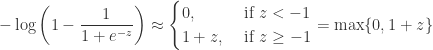
$(2y_i-1)\theta^TX_i > 1$ : Point is outside margin. No contribution to loss
$(2y_i-1)\theta^TX_i = 1$ : Point is on margin. No contribution to loss. As in hard margin case.
$(2y_i-1)\theta^TX_i = 1$ : Point violates margin constraint and contributes to cost.

Since the sum of non-negative convex functions is also convex, so the object function $J(\theta)$ defined above is convex, and it has a unique solution.

Gradient Descent Algorithm for SVM

Rewrite the optimization problem as an average format:

$\displaystyle \begin{aligned}\min_{\theta_0,\theta_1,...,\theta_n}J(\theta) &= \frac{\lambda}{2}||\theta||^2 + \frac{1}{m} \sum_{i=1}^m \max\{0, 1- (2y_i-1)\theta^TX_i\}\\ &= \frac{1}{m} \sum_{i=1}^m \left ( \frac{\lambda}{2}||\theta||^2 + \max\{0, 1- (2y_i-1)\theta^TX_i\} \right )\end{aligned}$

where $\lambda = \frac{2}{mC}$ is is the regularization parameter.

Therefore, the Gradient Descent update rule for SVM is:

Simultaneously Update:

$\displaystyle \theta_j := \theta_j - \alpha \frac{\partial}{\partial \theta_j}J(\theta_0, \theta_1, \theta_2, ...., \theta_n), j= 0,1,2,...,n.$

where $\alpha$ is the learning rate.

From the definition of the function $J(\theta)$ , it is easy to get:

$\displaystyle \frac{\partial}{\partial \theta_j}J(\theta) = \begin{cases}\frac{\lambda}{m}\theta_j + \frac{1}{m}\sum_{i=1}^m[-(2y_i-1)x_{ij}],&\text{ if } (2y_i-1)\theta_i^TX_i<1 \\ \frac{\lambda}{m}\theta_j,& \text{Otherwise } \end{cases}$

Database Oracle

The Trick of Retrieving the Saved Passwords From Toad for Oracle

September 10, 2014 lukelushu 8 Comments

In Windows 7, Toad for Oracle saves the connections and password in the files located in %USERPROFILE%\AppData\Roaming\Quest Software\Toad for Oracle\[version#]11.6\User Files\:

CONNECTIONS.INI
CONNECTIONACTIONS.INI
CONNECTIONPWDS.INI

Passwords are stored in encrypted way in CONNECTIONPWDS.INI file. If you forget the saved passwords for some Oracle users, you can retrieve them back from the encrypted PW file CONNECTIONPWDS.INI using the following tricky way.

The Trick:

Login in Toad as any user (has saved or not saved PW).
Choose Database|Create|DB Link menu item
Fill fields of the DB Link name, DB connection, and User to connect.
Then the password will be filled automatically if they are saved in the encrypted PW file before.
Click “Show SQL” button, the saved PW will be shown in the generated sql.

Try it!

	thx on The Trick of Retrieving the Sa…
	Jayron on The Trick of Retrieving the Sa…
	Abhirath Mahipal on Linear Regression with Multipl…
	zbra on The Trick of Retrieving the Sa…
	Bill Kuhn on The Trick of Retrieving the Sa…

Zero-Downtime Summary Table Refresh Using AB Rotating Tables in Oracle Exadata and Redshift

1. Zero-Downtime Refresh Framework in Oracle Exadata

2. Zero-Downtime Refresh Implementation in Redshift

S3 Folder Structure and Its Impacts for Redshift Table and Glue Data Catalog

Case 1: All the 4 files are in the root folder “test”:

Case 2: Some files are in the root folder and some files in subfolders:

Case 3: Files are in the same level subfolders:

Case 4: Files are in the different level of the multi-level subfolders:

Case 5: Files are in the same level of multi-level subfolders:

Conclusions

Redshift Naming Standard and Case Sensitivity

Standard Identifiers Rule

Double-quoted Identifiers Rule

Database Catalog and Reference of the Identifiers

Want to Return the Identifiers to Upper Case?

Examples

How to Assume IAM Role From AWS CLI

1. Grant an IAM user’s privilege:

2. Grant an IAM role to an IAM user:

3. Configure and use the AWS CLI profile to assume the granted role :

PL/SQL Wrap Utility for Encryption

Steps of Wrapping Packages/Procedures/Functions

Guidelines for Wrapping

Wrapping Oracle Views

Linear Separability: What is the best ?

Learning Maximum Margin with Noise

Possible Ideas:

Idea 1:

Idea 2:

SVM cost functions from logistic regression cost functions

Gradient Descent Algorithm for SVM

The Trick:

This blog will contain the technical notes for Oracle, Machine Learning, Quant tread, etc .

Linear Separability: What is the best $\Theta$ ?