Support Vector Machines is a widely used supervised learning algorithm to learn linear and non-linear functions.
Motivation
Classifying data is a common task in machine learning. Given a set of training data, each marked as belonging to one of two categories, and the goal is to decide which class a new data point will be in. In Support Vector Machines (SVM) training algorithm, a data point is viewed as a n-dimensional vector, and we want to know whether we can separate such points with a (n-1)-dimensional hyperplane, we call it a Linear Classifier. Ususally there are many hyperplanes that might classify the data. We can choose the best hyperplane as the one that represents the largest separation, or margin, between the two classes. That is, the distance from it to the nearest data point on each side is maximized. The SVM algorithm is to learn (find) such maximum-margin hyperplane or maximum-margin binary classifier.
Linear Classifiers and Margin
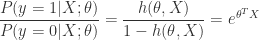
In Logistic Regression, we have the logistic regression hypothesis:
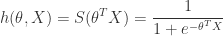
and make the following classfication based the estimated probability:
- When the probability of y =1 is greater than 0.5 then we can predict y = 1;
- Else we predict y = 0.
From the property of Sigmoid function, we can get the equivalent Linear Decision Boundary or Linear Classifier is:

Let us rewrite

Then the Linear Decision Boundary or Linear Classifier is

Now we can modify the Linear Classifier little bit by adding decision margins to get the SVM — We refer to SVM as a Large Margin Classifier:

- If
, we need
, not just
- If
, we need
, not just


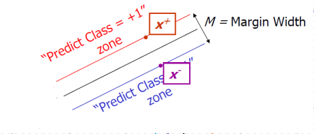
We can translate this Sigmoid function term into hyperplane language. If the training data are linearly separable, we can select two hyperplanes in a way that they separate the data and there are no points between them, and then try to maximize their distance. The region bounded by them is called “the margin”. These hyperplanes can be described by the equations
- Classifier Boundary:
- Plus-Plane:
- Minus-Plane:


Then the classification decision for a new coming example is:
- Positive Class (i.e.
): if
- Negative Class (i.e.
): if
How to Calculate the Margin Width
The distance between the Plus-Plane and Minus-Plane is called the margin width. How to calculate the margin width M in terms of 
From the Classifier Boundary equation 

Let
be any point on the Minus-Plane
be be the closest Plus-plane-point to
They are not necessarily example data points. Obviously, the vector 

Therefore, we have the following equations:
- 1.
- 2.
- 3.
(for some value k).
- 4.


Now it is easy to calculate the margin width 

and then applying the Eq.3, we get

So we have

Finally from Eq.4 we have


The datapoints lying on either the Minus-Plan or the Plus-Plan are called Support Vectors.
SVM – Optimization
Therefore, learning the SVM can be formulated as an optimization program: Search the
, if
, if


for 
We can compact this constraint as

Equivalently, from the margin width formula above, we have the optimization problem

s.t. 
This is a quadratic optimization problem subject to linear constraints and there is a unique minimum.
QP is a well-studied class of optimization algorithms to maximize a quadratic function of some real-valued variables subject to linear constraints (linear equality and/or inequality constraints). There exist algorithms for finding such constrained quadratic optima much more efficiently and reliably than gradient ascent method.
 .
.
 , but $ latex x^2$ will not work and it yields
  , since there are two spaces between $ latex and x_2 in the code. in the Text editor, it is OK to insert more spaces.


![\displaystyle \theta_0 := \theta_0 - \alpha\frac{1}{m}\sum_{i=1}^m[ h(\theta, X_i)-y_i]x_{i0}](https://s0.wp.com/latex.php?latex=%5Cdisplaystyle+%5Ctheta_0+%3A%3D+%5Ctheta_0+-+%5Calpha%5Cfrac%7B1%7D%7Bm%7D%5Csum_%7Bi%3D1%7D%5Em%5B+h%28%5Ctheta%2C+X_i%29-y_i%5Dx_%7Bi0%7D&bg=ffffff&fg=2b2b2b&s=0&c=20201002)
![\displaystyle \theta_j := \theta_j (1-\alpha \frac{\lambda}{m} ) - \alpha\frac{1}{m}\sum_{i=1}^m[ h(\theta, X_i)-y_i]x_{ij}, j= 1,2,...,n.](https://s0.wp.com/latex.php?latex=%5Cdisplaystyle+%5Ctheta_j+%3A%3D+%5Ctheta_j+%281-%5Calpha+%5Cfrac%7B%5Clambda%7D%7Bm%7D+%29+-+%5Calpha%5Cfrac%7B1%7D%7Bm%7D%5Csum_%7Bi%3D1%7D%5Em%5B+h%28%5Ctheta%2C+X_i%29-y_i%5Dx_%7Bij%7D%2C+j%3D+1%2C2%2C...%2Cn.+&bg=ffffff&fg=2b2b2b&s=0&c=20201002)
 is the learning rate and
  is the
  is often around 0.99 to 0.95. The second term is exactly the same as the original gradient descent.
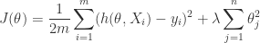
![\displaystyle J(\theta) = \frac{1}{m}\sum_{i=1}^m [-y_i\log (h(\theta, X_i))+(1-y_i)\log (1-h(\theta,X_i))] +\lambda\sum_{j=1}^{n}\theta_j^2](https://s0.wp.com/latex.php?latex=%5Cdisplaystyle+J%28%5Ctheta%29+%3D+%5Cfrac%7B1%7D%7Bm%7D%5Csum_%7Bi%3D1%7D%5Em+%5B-y_i%5Clog+%28h%28%5Ctheta%2C+X_i%29%29%2B%281-y_i%29%5Clog+%281-h%28%5Ctheta%2CX_i%29%29%5D+%2B%5Clambda%5Csum_%7Bj%3D1%7D%5E%7Bn%7D%5Ctheta_j%5E2&bg=ffffff&fg=2b2b2b&s=0&c=20201002)
 = \theta_0 + \theta_1 x_1 + \theta_2 x_2 + ....+ \theta_n x_n = \theta^TX") For Logistic Regression, we can resale the hypothesis
For Logistic Regression, we can resale the hypothesis![h(\theta, X) = S (\theta^T X) : \rightarrow [0, 1]](https://s0.wp.com/latex.php?latex=h%28%5Ctheta%2C+X%29+%3D+S+%28%5Ctheta%5ET+X%29+%3A+%5Crightarrow+%5B0%2C+1%5D&bg=ffffff&fg=2b2b2b&s=0&c=20201002)

![h(\theta, X) \in [0, 1]](https://s0.wp.com/latex.php?latex=h%28%5Ctheta%2C+X%29+%5Cin+%5B0%2C+1%5D&bg=ffffff&fg=2b2b2b&s=0&c=20201002) , we can interpret that value as the estimated probability that y=1 on input x for the give parameters
, we can interpret that value as the estimated probability that y=1 on input x for the give parameters 


![Image [5]](https://lukelushu.files.wordpress.com/2014/08/image-5.png)
 for the the linear hypothesis
 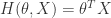 .
.

 .
.![Image [13]](https://lukelushu.files.wordpress.com/2014/08/image-13.png)
![Image [14]](https://lukelushu.files.wordpress.com/2014/08/image-14.png?w=235&h=221)


![\displaystyle J(\theta) = \frac{1}{m}\sum_{i=1}^m \text{Cost}(h(\theta, X_i),y_i)\\= -\frac{1}{m}\sum_{i=1}^m [y_i\log (h(\theta, X_i) ) - (1-y_i) \log (1-h(\theta, X_i))]](https://s0.wp.com/latex.php?latex=%5Cdisplaystyle+J%28%5Ctheta%29+%3D+%5Cfrac%7B1%7D%7Bm%7D%5Csum_%7Bi%3D1%7D%5Em+%5Ctext%7BCost%7D%28h%28%5Ctheta%2C+X_i%29%2Cy_i%29%5C%5C%3D+-%5Cfrac%7B1%7D%7Bm%7D%5Csum_%7Bi%3D1%7D%5Em+%5By_i%5Clog+%28h%28%5Ctheta%2C+X_i%29+%29+-+%281-y_i%29+%5Clog+%281-h%28%5Ctheta%2C+X_i%29%29%5D&bg=ffffff&fg=2b2b2b&s=0&c=20201002)

 :
: :
:![\displaystyle \theta_j :=\theta_j - \alpha \sum_{i=1}^{m} [h(\theta, X_i) - y_i]x_{ij}](https://s0.wp.com/latex.php?latex=%5Cdisplaystyle+%5Ctheta_j+%3A%3D%5Ctheta_j+-+%5Calpha+%5Csum_%7Bi%3D1%7D%5E%7Bm%7D+%5Bh%28%5Ctheta%2C+X_i%29+-+y_i%5Dx_%7Bij%7D&bg=ffffff&fg=2b2b2b&s=0&c=20201002)
 ,
,  ,
,  .
.
 be an (n+1)-dimensional vertical vector, where we always have
  as the “bias”, and
  are the n features (the n independent variables).
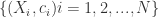
 be the dependent “target” variable.
 the training set with m examples. The i-th sample is
  , where
  is the j-th feature value.
 , where
  is the n+1 parameters to be determined, and


 , do the following until convergence:

![\displaystyle \frac{\partial}{\partial \theta_j}J(\theta)=\frac{1}{m}\sum_{i=1}^m[h(\theta, X_i)-y_i]x_{ij},j=0,1,2,...,n.](https://s0.wp.com/latex.php?latex=%5Cdisplaystyle+%5Cfrac%7B%5Cpartial%7D%7B%5Cpartial+%5Ctheta_j%7DJ%28%5Ctheta%29%3D%5Cfrac%7B1%7D%7Bm%7D%5Csum_%7Bi%3D1%7D%5Em%5Bh%28%5Ctheta%2C+X_i%29-y_i%5Dx_%7Bij%7D%2Cj%3D0%2C1%2C2%2C...%2Cn.&bg=ffffff&fg=2b2b2b&s=0&c=20201002)
![\displaystyle \theta_j := \theta_j - \alpha\frac{1}{m}\sum_{i=1}^m[ h(\theta, X_i)-y_i]x_{ij}, j= 0,1,2,...,n.](https://s0.wp.com/latex.php?latex=%5Cdisplaystyle+%5Ctheta_j+%3A%3D+%5Ctheta_j+-+%5Calpha%5Cfrac%7B1%7D%7Bm%7D%5Csum_%7Bi%3D1%7D%5Em%5B+h%28%5Ctheta%2C+X_i%29-y_i%5Dx_%7Bij%7D%2C+j%3D+0%2C1%2C2%2C...%2Cn.&bg=ffffff&fg=2b2b2b&s=0&c=20201002)


 to covert the Polynomial Regression into the Linear Regression problem with multiple variables
 .
. from the training set as the initial cluster centroids.
 .
. the index of k (from 1 to K) of the cluster centroids having the minimum distance (
 ).
). (for each class)
 mean of the examples assigned to cluster k
 be the index of cluster {1,2,…,K}. So the optimization objective of K-Means is:
 is the centroid to which the exsample
  has been assigned to.
 without changing the centroid
  .
.![Image [12]](https://lukelushu.files.wordpress.com/2014/08/image-12.png)
 . Where
  .
. be two points in
  . Then Minkowski distance of order p is defined as


